Free Download Project Management Spreadsheet Template

 Are you looking for a free, easy to use project management spreadsheet template? You've come to the right place. What are the benefits of using a project management template?

• Save time by using a pre-designed template to manage your projects and tasks.
  
• Helps project managers organize the project deliverables due from each working group, and track progress as it occurs
  
• Break down a large, complex project into numerous smaller, more manageable tasks.
  
• Consolidate all project tracking information in one location, and even break out individual areas for closer monitoring if necessary.
  
• Track each task and remain on schedule by using the project management spreadsheet template.

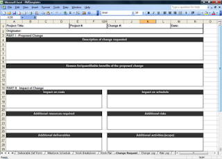
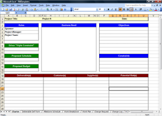
 The project management template includes: project charter, deliverable definition form, milestone schedule, work breakdown, work plan, change request, change log, risk log, an issue log, and more. Everything you need to successfully manage a project is included within this downloadable spreadsheet. Download today.

Note: The download link may require you to complete a survey before downloading the spreadsheet. If you would prefer to receive the Excel file as an email attachment please join my free Excel tips email newsletter.

Click to view my personal business project accounting and tracking spreadsheet tutorial.

UPDATE: For more templates visit my new page dedicated to project management.

Download a Gantt Chart Excel Spreadsheet Template

Are you looking for an Excel template of a Gantt chart? A Gantt chart is a graphical representation of the duration of tasks against the progression of time. This type of chart is a very useful tool for planning and scheduling projects and is helpful when monitoring a project's progress. You can use a Gantt chart to plan how long a project should take by laying out the order in which the specific tasks need to be carried out. Another major advantage of using a Gantt chart is that it lets you see immediately what should have been achieved at any point in time so you can take remedial action to bring a floundering project back on course. I have created a Gantt chart template in Microsoft Excel 2007. Please click the link below to download the spreadsheet.

EXCEL_Gantt.xls

*Enter to win a free copy of the Gantt Chart Template Pro.xls - a $39.99 value!

Visit our new page for more project management templates. 

Gantt Charts are extremely useful tools for planning and  project management and the Gantt Chart Template Pro from Vertex 42 is one of the best I’ve seen!

How do you avoid displaying errors in Excel spreadsheet formulas?

How do you avoid errors in Excel formulas? You don't need an online degree to figure this one out, but I do assume you have a basic understanding of simple logic formulas such as IF(). Sometimes, when you create a new formula you may get an error message in return (Here's a complete list of errors you may see in Excel: #N/A, #VALUE!, #REF!, #DIV/0!, #NUM!, #NAME?, #NULL!). In some cases, you'll want to know when a formula error occurs, but more often than not you would rather avoid these messages. You can do so by using an IF() function to check for an error. Use this standard format:

=IF(ISERROR(OriginalFormula),"",OriginalFormula)

For example, the formula below displays a blank if the division results in an error.

=IF(ISERROR(A1/B1),"",A1/B1)

 

Skip the Weekends Date Formula in Excel

I have a Date Started data in column A and Date Completed in column B. Column C I want to list how many days it took to complete the project so I subtract A from B (=B2-A2). However, I do not want to include weekends. So, if the start date is Friday and end date is Monday, currently my simple formula would display 4 days. I would like to create a formula that automatically skips over Saturday and Sundays, thus displaying the correct number of days as 2. How can this be accomplished?

Well, Excel actually has a built in function for this very reason. It is called NETWORKDAYS. It returns the number of whole workdays between two dates. To accomplish my task I simply use this formula, starting in cell C2: =NETWORKDAYS(A2,(B2-1)) Now you can calculate the number of work days there are between the start and end dates of a project by automatically excluding weekends. How cool is that?!

How do you change the default number of sheets in a new Excel workbook?

Every time you open a new workbook in Microsoft Excel, by default, it opens with three worksheets. You can, of course, insert more sheets or delete ones that you don't need. The good news is the unused sheets don't occupy additional memory or increase your file size, but if you are like me, the extra sheets just annoy me for some reason. I like to keep my workbook nice and clean. What can be done about this?

Well, you can actually change the default value of the number of sheets the Excel automatically opens with. How do you do this?

For Excel 2003: Go to: Tools>Options and click General in the Options dialog box. Next, change the setting for "Sheets in new workbook". Now all new workbooks will have the number of sheets you specify. I typically change this number to one unless I know I am going to have a monster spreadsheet.

For Excel 2007: Select the office window button>Excel Options. On the popup menu you will see the section "when creating new workbooks." Change the "include this many sheets" from three to whatever you desire.

How do you create a delete button for a form with a macro in Excel?

I managed to create a form to add records to a worksheet. Now what I want to do is add a 'Delete Record' button to the form to delete the last entry (or any other entry for that matter). First, how do you identify the entry you wish to delete? My solution is to use the first column as a reference column. Try using a macro like this:

Private Sub CommandButton1_Click()

Dim c As Long

Dim iRecord As String

Dim Deleted As Boolean

 

iRecord = InputBox("Enter Record Number to Delete")

c = Cells(Rows.Count, 1).End(xlUp).Row

Deleted = False

While Not Deleted

If Cells(c, 1) = iRecord Then

Rows(c).Delete shift:=xlUp

Deleted = True

End If

c = c - 1

If c <= 0 Then Deleted = True

Wend

End Sub

How do you flip or reverse a column of data in Excel?

How do you flip or reverse a column of data in an Excel spreadsheet? Well, if you simply want to reverse a list that's already in alpha or numeric order that is easily accomplished using the built in "Sort: feature (you can also easily transpose columns into rows and vice versa).

However, often you will find yourself with a column of data that isn't sorted (and may even be in different formats like a mix of numbers and text). How do you simply flip it so the bottommost items are on top and the top is now the bottom of the column of data?

There are a number of ways to do this, including writing a macro, but the easiest way I can think of is to simply create what I like to call a helper column. First, select the column you want to flip, right click it, and choose Insert to add your new helper column. Add a list of numbers starting with 1 and running down to the number of items in your list. Now select both of those numbers and then double-click the lower right corner of the cell that contains the 2 to quickly fill down the length of your target column.

Select your helper column and any other columns you want sorted along with it. Go to the Data tab and click the Sort button and use this to Sort by your helper column using A to Z or largest to smallest. That's it. Once completed, you can delete your helper column. Simple, eh?

Another more advanced method is to use a macro. Try this:

Sub FlipColumns()

Dim vTop As Variant

Dim vEnd As Variant

Dim iStart As Integer

Dim iEnd As Integer

Application.ScreenUpdating = False

iStart = 1

iEnd = Selection.Columns.Count

Do While iStart < iEnd

vTop = Selection.Columns(iStart)

vEnd = Selection.Columns(iEnd)

Selection.Columns(iEnd) = vTop

Selection.Columns(iStart) = vEnd

iStart = iStart + 1

iEnd = iEnd - 1

Loop

Application.ScreenUpdating = True

End Sub

 

Shared Apartment Expenses for 5 Roommates Spreadsheet

I recently updated my shared apartment expenses worksheet to account for up to five roommates. The purpose of this spreadsheet is to easily track who you owe money to. It's an easy way to divide up rent, cable, electricity, groceries and random other oddities. The instructions are included with the spreadsheet. You can download the shared expenses workbook here.


Shared Apartment Expenses for 5 Roommates Spreadsheet.xls

How do you change the worksheet tab color in Microsoft Excel?

 Excel 2003 Users


If you are wondering how you change the worksheet tabs color in an Excel spreadsheet then the title of this post might be a little deceiving. Unfortunately, this feature is not currently available in Microsoft Excel. It would certainly be helpful to many users to be able to color-code your worksheet tabs. For some unknown reason, Microsoft hasn't implemented this feature yet although I hear it has been available in 1-2-3 and Quattro Pro for quite a while. Still, that's not enough to make me quit using Excel and switching to another program. 

Excel 2007 Users

You can easily change the tab color in Microsoft Excel 2007 by going to the home tab, clicking on the Cells section, going to Format and then hit "Change tab color." Easy. 

How do you capitalize letters in a name with Excel VBA macro?

Is it possible to have a VBA macro capitalize the first letters in someone's name? For example, if a name is John Stoneburner and a user only enters "john stoneburner' in a text box could it would automatically capitalize it to be John Stoneburner. With Excel, anything is possible! There are two options you could try:

Dim myString as String
myString = Application.WorksheetFunction.Proper(TextBox1.Value)

Or use this option:

Range("A1") = UCase(Left(Range("A1"), 1)) & Mid(Range("A1"), 2)

Honeymoon vacation planner spreadsheet template suggestions?

	Budget
Hotels	---
Airfare	---
Car Rentals	---
Activities	---
Meals	---
Petrol	---
Misc.	---
Total	$0.00

 

I am working on changing the Excel spreadsheet I used to help plan my honeymoon vacation into a downloadable user template. Here are the major categories I have listed to help users plan their budgets and activities. Are there any categories that I am missing that you would like to see added? I'm sure I will be able to add more unexpected items after I go on my actual honeymoon.

Booked	Item	Cost	Budget	Balance
YES	Hotels	$1,511.83	---	#VALUE!
YES	Airfare	$600.80	---	#VALUE!
SELECT	Activities	$874.00	---	#VALUE!
SELECT	Car Rental	$279.13	---	#VALUE!
SELECT	Meals		---	#VALUE!
SELECT	Petrol		---	#VALUE!
SELECT	Misc.			$0.00
	Total	$3,265.76	$0.00	#VALUE!

Looking for an Excel Football Schedule Spreadsheet Template?

Fall is upon us and you know what that means- it's football season! Whether you're following your son in middle school, your high school, a college team, or a fantasy NFL team, an Excel spreadsheet is a good way to keep track of your favorite team's stats. Here is a spreadsheet I put together as a quick example. Column A is for the week number of the season. Column B is to list your favorite team. Column C is for their schedule, who the opponent is every week. Next, D is your team's score and E is your opponent's score. Up to this point all the columns have required manual data entry. The next columns are all formulas.

 Column F is the result column, a Win, a Loss, or a Draw. I used a simple IF formula: 

=IF(D2>E2, "W", IF(D2

Next, I want to know what the current winning or losing streak is. I insert a column with the following formula starting in cell G2:

=1+(IF(F3=F2,G2,0))

Now in the streak column I can use a simple concatenate: 

=F2&G2 

Now, for a complete football stats page I want to see what my team's overall record is. To do that I use this formula:

=COUNTIF(F:F, "W")&"-"&COUNTIF(F:F, “L")&"-"&COUNTIF(F:F, "D")

 

Winning percentage is another easy formula and useful stat.

=COUNTIF(F2:F11, "W")/COUNTA(F2:F11)

 

The remaining statistics are all simple average, max, and min formulas. Take control of your fantasy football league with the football schedule Excel spreadsheet! What other stats or features would you like to see on my football template spreadsheet?


Download Football Schedule Spreadsheet.xls now!

How do you get Excel to recognize milliseconds?

I recently needed to import some elapsed time data from a scientific instrument into Microsoft Excel for in order to compute some complex calculations. The scientific instrument provided elapsed time in the following format:

01:02:03:123 where 01 = hours, 02 = minutes, 03 = seconds and 123 = milliseconds.

At first glance, Excel does not seem to recognize milliseconds. However, you just have to know what Excel is looking for. In this case, Excel expects to see milliseconds as:

01:02:03.123

Notice the difference? It is tiny yet important (a "." instead of a ":").

 

Another method to recognize milliseconds in Excel may be to try this formula:

=REPLACE(A1,9,1,".")+0 where your time values are in column A. Then, format the converted values as hh:mm:ss.000

How do you create bullet points in Microsoft Excel 2007?

How can you do bullet points in Excel similar to those in Microsoft Word? There are at least six methods that I know of:

1. =CHAR(149)

2. Alt+0149

3. Alt+249

4. The lower case letter n in Wingdings font

5. You can also import them from Word or use the character map (char.exe)

6. VBA code line: ActiveCell.Value = "•"

There may be others that I haven't thought of yet. Any suggestions?

How do you copy and paste cell value only with VBA in Excel?

I was recently asked this question: Is there a way in Excel to write a macro to copy a cell's numeric value only and not the formula? Basically, can you use VBA to paste only the value, like the Paste Special feature in the Values Only menu? The answer is yes!

To do a simple Paste operation you might write this line of code:
ActiveSheet.Paste Destination:=Worksheets("Positions").Range("A2")

Instead of '.Paste', use '.PasteSpecial." Try it with this line:
Worksheets("Positions").Range("A2").PasteSpecial xlPasteValues

If you still have questions then see the Microsoft Excel VBA help file for the use of the PasteSpecial method. It's pretty straightforward.

Another suggestion, instead of using code like this:

Set rng6 = .Range("A3").End(xlDown).Offset(0, 41)
rng6.Copy
ActiveSheet.Paste Destination:=Worksheets("Positions").Range("A2")


you could use something like this:

Worksheets("Positions").Range("W2").value = .Range("A3").End(xlDown).Offset(0, 41).value

This new code will accomplish the same thing as the original but it will also allow your code to run more quickly by avoiding the use of copy and paste althogether.

Where can I download the roommate's shared apartment expenses spreadsheet?

My shared apartment expenses spreadsheet has become very popular and I have received a lot of positive feedback. Many people have emailed me or commented on this blog and I've sent each request a copy of the spreadsheet. Still, I get the feeling that a lot of readers are a bit apprehensive about posting their email addresses here. I would never give that information away but anyone reading the comments could. Therefore, I have finally decided to find a site where I can post my Excel files for easy download. Here is the link for the latest version of my shared apartment expenses spreadsheet for those of you with roommates. In the coming days I will be posting more of my templates. Any requests?

Shared Apartment Expenses Spreadsheet.xls

Some lesser known keyboard shortcuts in Microsoft Excel

Here are a few shortcuts in Microsoft Excel that you may not be familiar with:

Alt+F11:Open VBE
Ctrl+Shift+Enter:Array formula
Ctrl+F3:Define name
F3:Paste name
Ctrl+Spacebar:Select columns
Shift+Spacebar:Select rows
Ctrl+1:Format cells
Ctrl+B:Bold
Ctrl+U:Underline
Ctrl+:Current date
Ctrl+shift+:Current time

File this one under "what are some keyboard shortcuts in excel?"

Where can I download an Apartment Search Spreadsheet ?

My apartment search spreadsheet has become very popular and I have received a lot of positive feedback. Many people have emailed me or commented on this blog and I've sent each request a copy of the spreadsheet. Still, I get the feeling that a lot of readers are a bit apprehensive about posting their email addresses here. I would never give that information away but anyone reading the comments could. Therefore, I have finally decided to find a site where I can post my Excel files for easy download. Here is the link for the latest version of my apartment search spreadsheet. In the coming days I will be posting more of my templates. Any requests?

Apartment Search.xls

How do you transpose a column into a row with a formula in Excel?

It's easy to copy and paste data to turn vertical columns into horizontal rows. But sometimes you may want to automate this task. You can use array formulas to transpose lists of data.  Transposing a range means turning a row into a column, and turning a column into a row.  In other words, it rotates the orientation of the data by plus or minus 90 degrees. You can reverse the order or keep it the same.Here's how to do both:


How to transpose a column Into a row with the same order:

These functions will transpose a column list, CList, into a row.  To keep the data in the original order, create a named range called RList referring to the cells in a row that is to contain the transposed data.  Then use the following array formula: 


=OFFSET(CList,COLUMN()-MIN(COLUMN(RList)),0)

How to transpose a column Into a row with the REVERSE order:

To reverse the order, create the named range "RevRList" then enter this formula:

=OFFSET(CList,MAX(COLUMN(RevRList))-COLUMN(),0) 

Personal Online Finance Tracker Excel Spreadsheet Template

I'm going to try and post more templates seeing how my apartment search spreadsheet has been such a big hit. With economy still in the crapper and questionable job security many Americans, including myself, have turned towards the internet for a source of additional income. How do you make money online? Well, this blog, as well as several other blogs that I have created are a great place to start. Then there are online surveys, selling stock pictures, writing articles, and even getting paid just to receive a couple junk emails a day. So how do I organize all of these methods in order to keep track of my finances and maximize my time? Excel spreadsheets of course!

As you can see, I started this money making endeavor in December of 2009. I've listed across the top row all of my sources of income, followed by the total and a few statistics. Here are the formulas I used:

Total: =SUM(C2:Q2)
Days: =IF(--TEXT(TODAY(),"yyyymm")>S2,DAY(DATE(2010,2,0)),DAY(TODAY()))
Ave/Day: =R2/T2
Ave/Blog: =U2/4

This formulas are pretty straight forward:

Have you ever wondered how much money the ads displayed on this site bring in? Well, now you will know. Google Adsense plus Kontera Ads = $50 over 6 months, or about 15% of my total online revenue.

Survey sites, including MySurvey and Opinion Outpost have netted over $150, almost half of all my online earnings.

Writing articles for WikiNut has been fun but not very profitable- yet. Sometimes it takes time to build up an audience of followers and dedicated readers. I remain optimistic on this one for the future.

You can sell pictures online at sites like Dreamstime to try and make a few bucks.

I recently started reading emails for a few cents a day with sites like Send Earnings and Inbox Dollars. They won't help you get rich quick but if you keep at it you can have a nice, steady growth.

My projected earnings for the year right now are around $700. You won't get rich quick but you can easily make some extra spending money. Every little bit helps in this economy!

How do you assign a letter grade to a number in an Excel spreadsheet?

A frequently asked question is how do you assign a letter grade to a numeric value.  This is actually very simple.  First, you need to create a defined name called "Grades" which refers to the array:

={0,"F";60,"D";70,"C";80,"B";90,"A"}

Next, use the VLOOKUP function to convert the number to the letter grade:

=VLOOKUP(A1,Grades,2)

In this case, A1 is the cell that contains the numeric value.  You can add entries to the Grades array for other grades like C- and C+, just make sure the numeric values in the array are in increasing order.

Also, I am currently planning for my honeymoon so what I have turned to in order to keep my notes and thoughts organized? Excel spreadsheets of course! So stay tuned for my Honeymoon/vacation planning/budgeting Excel spreadsheet.

How to find the most common name in an Excel spreadsheet?

How do you find the most common name or string in a range in an Excel spreadsheet? The following array formula will return the most frequently used entry in a range, where Rng is the range containing the data:
 
=INDEX(Rng,MATCH(MAX(COUNTIF(Rng,Rng)),COUNTIF(Rng,Rng),0))

How do you counting characters in a string in Excel?

I found this to be a very useful little function. This is one of those formulas that is easy but most people may not know it so maybe you can impress your boss with it one day. The following formula will count the number of "B"s, both upper and lower case, in the string in B1.

=LEN(B1)-LEN(SUBSTITUTE(SUBSTITUTE(B1,"B",""),"b",""))

Shared Apartment Expenses Spreadsheet Template

Where can I find a copy of a shared living space expenses spreadsheet template? Right here of course! I've created a new template for my Shared Apartment Expenses spreadsheet. Please email or comment if you would like a copy. This is the first version of this document. I could use some good feedback while I am improving and working on a new version. Is it easy to use? Are there any features you would like to see added? Do you care about the statistics or not? This is a good companion spreadsheet to my Apartment Search template.

Updated Apartment Search Spreadsheet

Based on recent users suggests and feedback I have made a few additions to my Apartment Search Spreadsheet. Many of these suggestions I had never heard of before, mainly due to the fact the reader lives in a different geographic region than I do. The following is the complete list of additions:


-Added "Gym / Fitness Center" to the Yes or No options. Duh. Can't believe I forgot that obvious one.

-In the input info, added rows for "Square Feet (Bedroom 1)", "Square Feet (Bedroom 2)", "Square Feet (Bedroom 3)", "Square Feet (Living Room / Dining Room)". The reason for this is that if you are sharing an apartment with roommates they may have a different requirement for bedroom space.
 

-In move-in fees, I added "Credit Check Fee". In the states, it is very common for landlords to charge a nominal fee to check a prospective tenant's creditworthiness (cool word bro, creditworthiness).
 

-In some major metropolitan areas, such as New York City, it is very common to install a pressurized wall in a bedroom or living room so you can squeeze one more person into the apartment and decrease living costs. Usually these walls are leased, as they are temporary and must be removed before the lease is up. Sometimes they aren't even allowed. Thus, I added a "Pressurized Wall Lease / Month" in Monthly Expenses, "Pressurized Wall Installation Fee" in move-in fees, and "Pressurized Wall Allowed" in the Yes or No Options.
 

-I also added a "Rent Controlled" in Yes or No Options. Some apartments are rent-controlled to protect tenants from massive rent increases when their lease is up and they wish to renew. Of course, these apartments are extremely coveted. There are other places which have rent-controlled apartments, but apparently New York City is the most well known for it.


Hopefully now the apartment search spreadsheet can accommodate an even larger percentage of the population and address each individual's needs. Do you have any other suggestions? As usual, email me or comment below for your copy of this latest version of the Apartment Rating/Search Spreadsheet.xls.

New Apartment Search Rating Spreadsheet

I recently completed a new and improved version of my Apartment Search Spreadsheet. Please leave a comment or email me if you would like a copy. The instructions are included within the spreadsheet. I would appreciate any feedback you have: is it easy to use, is there any information missing, anything suggestions you have to make it better.

This rating spreadsheet utilizes a simple house of quality to give each potential apartment an overall score based on several factors in which you give an importance rating. This way, items that are important to you contribute more to the overall score if they meet your requirements. I've tried to make the process as simple as possible through the use of drop down lists.

Also, I am putting together a job search spreadsheet. I need your help. What are some items you would like to see on this spreadsheet template? I have listed a few already such as: distance to home, salary expectations, relocation paid for, etc. What other information are you most interested in when searching for a new job and to help keep it organized?

How do I clear rows in Excel spreadsheet with a macro?

Do you have a huge spreadsheet with a ton of rows that you need to delete each time you use it? Here is a simple macro to help you. This is for a spreadsheet that is password protected. Now, I have headers in row 1 and formulas starting in row 2 that I don't want to wipe away so I select the range starting in row 3.

Sub Clear_Rows()

''' Protect User Interface Only '''

ActiveWorkbook.Sheets("sheet1").Activate

Sheets("sheet1").Protect Password:="pass1", UserInterfaceOnly:=True

 

''' Clear Rows '''

Range("a3:xfd1048576").Select

Selection.ClearContents

Range("a1").Select

End Sub

How do I save an Excel file with a macro?

There may be times when you will want a macro to save a file automatically after it is run. The second macro will save the file with a name called "MySavedFile". You may specify the path if you need to. The last macro saves all opened workbooks.

Sub SaveFile()
ActiveWorkbook.Save
End Sub

Sub SaveName()
ActiveWorkbook.SaveAs Filename:="C:\MySavedFile.xls"
End Sub

Sub SaveAll()
myFile = ActiveWorkbook.Name
    ActiveWorkbook.Save
    ActiveWindow.ActivateNext
Do While mySavedFile <> ActiveWorkbook.Name
    ActiveWorkbook.Save
    ActiveWindow.ActivateNext
Loop
End Sub

Shared Apartment Expenses Spreadsheet

Have you ever been in that situation where you are sharing a living space with a number of other people and you are constantly trying to figure out who owes who what because each utility is in a different person's name? I've moved fourteen times in the past six years (because of going back-and-forth from university to co-op every semester) and I've had different roommates at each location. I needed a quick and easy way to keep track of who owed me money or what I owed someone else and to make sure all the bills were paid. I wanted this to stay updated in real time so I could simply look at it whenever and know exactly what was due and who to pay, all without needing to sit down do the math every time. This has lead to the creation of my Shared Apartment Expenses Spreadsheet. The following example is for an apartment with three roommates.

The first thing I do is list a description of what utility or rent is due. In the next column I list the amount due. The next column is the category where the expense falls under. These are actually drop-down lists which originate on another sheet where I listed out all of the possible categories. See data validation if you don't know how to make a drop down list. I only did this so I could look at statistics for each month and category.

I also put the due date for each bill and when it was actually paid for my records. Now the important part: who paid what? I make a column for each person and every time they pay a bill I put the amount under their name next to the item that they paid. 

The next section is who owes who what. Now this could be a simple formula if you have decided to split everything evenly among yourselves. But come on, life is never that simple. The apartment I am living in has a one car garage and a master bedroom. It's not really fair to the person that gets screwed out of the garage and doesn't even get their own bedroom! Therefore, we decided to split the rent like so: 

  Instead of having a simple formula you have to manually enter the amounts for the rent. Every other utility is split evenly. The totals are listed at the bottom of the columns. Now, the next thing we want to prevent is to have to write a million checks. If you owe me money, but I owe you more money, I simply subtract what you owe me then write you a check. 

Next is the all important who paid what. This is more complicated and confusing the more people you have but it works and in the end makes things much easier. I list each person and what they've paid to the other two people. I then add up the total at the bottom.

Alright, so that's the easy and obvious part but I want to know what the balance is right now. Below the who paid what section is where the magic happens. First, in cell R16 I take what Nick owes Brian and subtract what Nick PAID Brian (=K12-R12). In the next cell I take what Nick owes Ron and subtract what Nick PAID Ron (=L12-S12) and so on for the other two people. Now we can see who owes who what after payments. Brian owed Nick $86.71 but after a payment of $22.16 only owes him $64.55.

However, Nick also owes Brian $31.67, which is less than what Brian owes Nick. So, we subtract what Brian owes Nick so that Brian just has to pay Nick $32.88 instead of $64.55. Make sense? The formula looks like this: 


=IF(R16>T16,R16-T16,0)


If what Nick owes Brian is greater than what Brian owes Nick, subtract the two, otherwise put zero. Nick's balance for Brian is zero. Brian's balance is greater than Nick's so subtract the two and get $32.88. Basically, each person either has a zero balance or they owe money to someone. There should be no negative values.

The last line tells you who you owe money to in real time. Every time someone makes a bill payment or pays someone else it automatically updates and adjusts the values. No math involved! No more fighting over who paid what and when.

On the last sheet (Statistics) I decided to get a little crazy and keep track of some statistics: the totals for each month and which utility was the biggest drain on my wallet. I used this formula for the utilities

=IF(Statistics!B$1=Balance!$C4,Balance!$B4,"")


And this formula for the months: 


=SUMIF(Balance!D:D,A15,Balance!B:B)

This is also a good place to check the totals with the master sheet to ensure your work is correct.

I had to make some quick graphs to visualize the data. Who doesn't love a good pie chart? 

And there you have it, another practical, real world application of Microsoft Excel!

 

 

 

 

Excel Spreadsheet Macro: Highlight Duplicates

This is a simple yet effective macro for your Excel spreadsheet. There are times you need to highlight duplicate data in your worksheet. You could use the duplicates function but that actually ends up deleting everything that is a duplicate. Sometimes you may just want to point out what is a duplicate and not physically delete that data. This macro is what you could use instead.

Sub DupinRed()
Application.ScreenUpdating = False
Rng = Selection.Rows.Count
For i = Rng To 1 Step -1
myCheck = ActiveCell
ActiveCell.Offset(1, 0).Select
For j = 1 To i
If ActiveCell = myCheck Then
Selection.Font.Bold = True
Selection.Font.ColorIndex = 3
End If
ActiveCell.Offset(1, 0).Select
Next j
ActiveCell.Offset(-i, 0).Select
Next i
Application.ScreenUpdating = True
End Sub

How do I create a ratings system in Excel?

Normally, this blog is about me trying to help you with Excel spreadsheets. Well today, maybe you can help me. I am trying to come up with a new rating system in Excel. I don't want this to end up being a popularity contest, so I want to use experience as a criteria too. Users will rate an item A through F (could be anything from restaurants to roller coasters) with a value of 1 to 5, 1 being lowest and 5 being highest. Not every user will rank every item, only the ones they have ever experienced. To account for this I have a user experience index. I counted the total number of items experienced by each user, ranked them in reverse order, then divided by the total number of users (in this case there are 5). Thus, each users experience index is between 0 and 1, with 1 being the most experienced user.

I also wanted to incorporate a popularity index. I count how many users have used each item, rank them in reverse order, then divide by the total number of items. The popularity index is between 0 and 1, with 1 being the most popular item.

So now that I have this data I am not sure what to do with it. How can I combine them in a meaningful way? I've tried this formula:

(User rating * user experience index)/SUM(user experience index) * popularity index

The problem is probably with the popularity index. With it being linear, it gives far too much advantage to the most popular items, and goes too far to penalize those that don't see as much action. It over-compensates for the problem I described. I don't remember anything from the one statistics class I took in college so I'm not sure what to do. It feels like the linear experience index actually works really well, it just seems like the popularity index is off.

Any suggestions?

NCAA Bracket Madness by David Tyler

We have a special treat for you today. Our very first guest blogger is David Tyler, the creator of what I consider to be the best March Madness Excel bracket on the internet, as I stated in a previously. I really appreciate David taking the time and sharing his insight, experience, and wealth of information with us today. Now, on to the article!
 -------------------------------------------------------------------------------------------------------

Every March, thousands of people fill out NCAA basketball tournament brackets, for which someone is faced with the challenge of running the pool.  This process can be tedious and fraught with human error.  To alleviate this, we can use a two-file Excel solution: a Bracket file submitted by all pool participants, and a Pool Manager file used to track the results once the tournament has begun.

Nick asked me to provide a brief posting on how these files work.  Below is a basic overview, but I recommend poking around the files to learn more.  Please bear in mind that the bracket files aren't perfect, and there are better ways that I've often been too lazy to implement, but the current files serve their purpose.

The Brackets

Most importantly: we need good, clean data.  Let's say there is a game involving Massachusetts.  If the participant puts the winner as "UMass," a human understands what that means, but Excel doesn't.  The file needs to have "Massachusetts" exactly.

To keep data consistent, all participants must submit the exact same bracket file.  By using VBA code that allows the user to click on a cell to advance that team, there is no opportunity for mis-typing.  The user clicks on "Massachusetts" in cell B4 and it automatically advances the cell's contents ("Massachusetts") to cell C5.  The user sees this as a quick and easy way to fill out a bracket; in reality, its main purpose was to help ensure good data.

For users who don't/can't enable macros, the file also uses a combination of Data Validation, formulas, and Conditional Formatting to ensure clean data.  Having alternative checks is an important component to maintaining clean data.  Many thanks to my friend Tom Szarek for the clever design of these great VBA-free features.

Collecting the brackets

With everyone using the same bracket file, we always know what data is going to be in which cells - e.g., C5 will always have the winner of the upper-left region's 1-16 matchup.  This allows the Pool Manager file's VBA code to open a participant's bracket (previously saved off to the pool administrator's hard drive), store the picks in an array, and then write those picks at a row of data in the Pool Manager file.  This is automatically repeated for all participants, storing all pool participant data on the same worksheet.  At this point, the Bracket files are no longer of any use.

Evaluating the brackets

Using formulas, we compare the actual winners of the games (from the MasterBracket tab) with the participant's picks.  If 'actual winner' on MasterBracket = the 'pick' on the Picks tab, the participant earns the points from that game.

The participant score is computed instantly with formulas on the Leaders tab.  VBA then sorts the leaderboard in descending order so the highest scorer is on top.  The resorting could be done with some array formulas, similar to those used on the PartInfo tab, but VBA is easier and less resource intensive.

Enjoy March!

Any time you are doing the same task multiple times, you need to question how Excel and VBA can be used to reduce the workload.  With these files, pool administrators can handle a large number of participants with little additional effort.  Further, once the Pool Manager file has all data, the administrator can send the file to all pool participants -- this lets participants track scores on their own, generate scenarios, and see other pool participants' picks.  The less time spent on administration, the more time there is to enjoy the games and the taunting of friends in the pool.

----------------------------------------------------------------------------------------------------------

That was great David, very informative, especially the part about reducing the workload when working with repetitive tasks. I've found that to be very true in my engineering work experience. Thanks again for sharing with us. Don't forget to check out David's blog here.

We're always looking for innovative and unique features and spreadsheets utilizing Microsoft Excel so please don't hesitate to contact me with your ideas or if you are interested in guest blogging.  Thanks for reading.

How do I make horizontal rows into vertical rows in Excel Spreadsheet?

To make horizontal rows into vertical columns, highlight the cells you want to change, copy, right click cell you want to move to, select ‘paste special’, click ‘transpose’ box, hit ok. It's that simple!

Join our free email newsletter for more advanced Excel tips to make your life easier! Don't worry, we won't swamp your inbox and you can unsubscribe at any time. We'll even send you some useful Excel templates from time to time. Cheers!
 

What’s the best 2010 NCAA Excel Bracket?

March Madness is here! Are you looking for a great way to start an NCAA Basketball Tournament pool with your friends or coworkers? After downloading several different Excel spreadsheet brackets I think I have found the best one.

http://whenthewhistleblows.wordpress.com/2010/03/08/ncaa-basketball-march-madness-excel-brackets/

Through the use of several macros, the bracket is very easy to use and has a very clean appearance (much more so than most of the other Excel brackets that I downloaded). You can even create html pages to post on the web the current standings. Download it and see for yourself!

 

(Note: there are two files to download, the blank bracket to distribute to all of your friends plus the Pool Manager to keep track of all your scores. Instructions are included!)

How do I insert the degree symbol in Microsoft Excel? (And other keyboard shortcuts)

There are a number of keyboard shortcuts that can be used to generate symbols in Excel spreadsheets. The most asked about one is how to insert the degree symbol. Here is a list of some of the most frequently used keyboard shortcuts:

Alt + 0176 = ° (Degrees)
Alt + 0149 = • (Bullet)
Alt + 0162 = ¢
Alt + 0188 = ¼
Alt + 0189 = ½
Alt + 0190 = ¾
Alt + 0177 = ±
Alt + 0178 = ²
Alt + 0179 = ³
Alt + 0163 = £
Alt + 0128 = €
Alt + 0151 = — (m dash)
Alt + 0150 = – (n dash)
Alt + 0187 = »
Alt + 0169 = ©
Alt + 0174 = ®
Alt + 0165 = ¥
Alt + 0177 = ±
Alt + 0247 = ÷
Alt + 0166 = ¦
Alt + 0134 = †
Alt + 0227 = ã
Alt + 0191 = ¿
Alt + 0161 = ¡
Alt + 0209 = Ñ
Alt + 0241 = ñ
Alt + 0225 = á
Alt + 0233 = é
Alt + 0237 = í
Alt + 0243 = ó
Alt + 0250 = ú
Alt + 0252 = ü
Alt + 0186 = ° (1° = primero)
Alt + 0170 = ² (2² = segunda)

As with most software these days, there are a number of different ways to get to the same result. You can also use character map to use the symbol you are looking for:

A character map of all special symbols, including foreign language characters, can be displayed by going to Start>Run, typing charmap, and clicking OK (Windows XP users). Vista users will type charmap into the Search window at the bottom of the Start Menu. Choose the font corresponding to the one you're using and click on a character. Next click Select>Copy to copy the character. Return to your document, click where you want the character inserted, and go to Edit>Paste (or do Ctrl+V) to insert it.

Finally, the simplest way is simply to where MSOffice users can go to Insert>Symbol to accomplish the exact same thing.

How do you automatically enable macros when Excel is opened?

•To automatically enable all macros when Excel is opened so you don’t have to do it manually every time, please read the following instructions:

1. In Excel, click the Office button in the upper left corner of the screen. 

 

  2. Click the "Excel Options" button in the lower right.

  

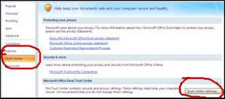
3. Click the "Trust Center" button on the left. Then, at the bottom right, select "Trust Center Settings" as shown below.

 

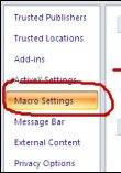
4. In the next window, select "Macro Settings," then select the radio button for “Enable all macros."

 

  There you have it! Now you don't have to enable the macros every single time that you open Excel.