Sunday, February 26, 2017

How to check if sheet name exists with VBA

In Excel, you can't have two sheets with same name in the same workbook. If you create a copy of a worksheet, Excel will automatically rename the sheet, usually adding a (1) onto the name. Try creating a copy of an existing sheet and see for yourself. As you add more sheets you probably want to rename them to keep your spreadsheet organized.

There are times when you are using a VBA macro to automate processes in Excel when you want to rename a sheet. If the new name of the sheet is unique your program will be fine. However, if the macro tries to rename a sheet with a name that already exists as another sheet name, you could have a problem. One way to avoid this to make your macro more robust is to add code to loop through all the sheet names and check to see if your new sheet name already exists, and if it does then add something onto the name to make it unique.


Sub CheckSheetNames()

Dim i As Integer
Dim y As Integer

‘the new sheet name, what I want to rename the active sheet as
Dim myName As String
myName = "Sheet"

y = 0

‘loop through all the sheets in the activeworkbook
For i = 1 To ActiveWorkbook.Worksheets.Count

‘if my new sheet name matches any of the existing sheet names, then increase the y count by 1
If myName = Left(ActiveWorkbook.Worksheets.Item(i).Name, 5) Then

y = y + 1

Else
End If

Next

‘If y is greater than 0 then we know that a sheet already with that name already exists
If y > 0 Then

ActiveWorkbook.ActiveSheet.Name = myName & “(“ & y & “)”

Else
‘if y is 0 then the sheet name does not exist so we are free to rename it
ActiveWorkbook.ActiveSheet.Name = myName
End If
End Sub


Now you know how to automatically rename worksheets and how to loop through sheets using VBA. Adding simple checks like these will make your code better and more robust, so if others are using it that don’t have any programming experience they are more likely to not encounter any errors.

Tuesday, February 21, 2017

How to link a textbox to a cell Excel Macro

If you’re putting together some kind of diagram in Excel, you may want to have the ability to click on a shape or textbox and have it automatically jump to another location, like a cell. I have always believed it is faster to mass produce things then manually delete what you don’t need rather than manually creating textboxes, and this is another example of that. I would run a macro to create 50 linked textboxes and then if I only use 30 I can quickly delete the left over 20.
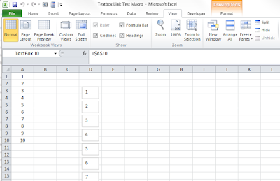
For example, the macro creates ten Textboxes and then links them to cells A1 through A10 using an automatically created hyperlink. The two most important expressions we will be using are:
To add and position a new Textbox using VBA:
.AddTextbox(Orientation, Left, Top, Width, Height)
To add a hyperlink to a textbox using VBA:
.Add(Anchor, Address, SubAddress, ScreenTip, TextToDisplay)
How to link a shape to a cell Excel Macro

If you’re not familiar with programming VBA macros in Excel, check out my quick start guide here. Listed below is the complete code with my comments to help walk you through it:
Sub CreateTextBoxes()
Dim i, d As Integer
‘d will be used as spacing to separate the textboxes so they are not created on top of one another
d = 10
‘perform the loop 10 times and create 10 textboxes. Could change this to be more or into a user input box
For i = 1 To 10
'create textboxes in a vertical column with equal spacing using d
       ActiveSheet.Shapes.AddTextbox(msoTextOrientationHorizontal, 150, 20 + d, 35, 25).Select
   
'add formula to textboxes so the textbox displays the text in the cell
    Selection.Formula = "=$A$" & i
   
'create hyperlink from textbox to cell, assumes sheet name is Sheet1
       ActiveSheet.Shapes.Range(Array(i)).Select
    ActiveSheet.Hyperlinks.Add Anchor:=Selection.ShapeRange.Item(1), Address:="", SubAddress:="Sheet1!A" & i
   
    d = d + 30
  
Next
End Sub

How to link a shape to a cell Excel Macro Video


If you put some values in cells A1 – A10 and then run this macro, it will create 10 textboxes, and when you click on the textbox it will jump to the location of the appropriate cell.  Download this sample file here.

Thursday, February 9, 2017

2017 NASCAR Fantasy League Manager Spreadsheet

2017 is the fourth year in a row that I’ve made the NASCAR Fantasy League spreadsheet available for download. This NASCAR fantasy game is based on Total Driver Points according to NASCAR’S scoring system. In order for your drivers to score they must be running for Monster Cup Points. Drivers may run in more than one NASCAR division but can only score points in one division.


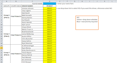
2017 nascar fantasy league manager in excel


How to Play NASCAR Fantasy in Excel


At the beginning of the year (first race is Daytona on February 18th) participants choose ten race car drivers. These will be their 10 drivers for the entire year - no changing after the entry deadline. All players also submit the three drivers that they think will place 1st, 2nd, and 3rd in the NASCAR standings at the end of the year. They don’t need to have these drivers in their picks, just who they think is going to finish on top. This is used as a tie-breaker.

The fantasy league manager manually enters each player’s picks into the spreadsheet at the beginning of the year (or uses the new entry form to copy and paste entries). Players keep the same drivers all year long. After each race, the manager then goes to ESPN.com and enters the amount of points that each driver earned during the race into that driver’s column. The spreadsheet then automatically adds and ranks each player according to their driver’s scores. I used many of the same formulas found in the leaderboard of my NCAA Bowl Prediction Pool sheet. This NASCAR fantasy manager template can currently handle up to one hundred drivers and one hundred participants without needing to modify a single formula!


This year, there are two options to download the 2016 NASCAR Fantasy League manager:


Download Option 1 (no email required)


Simply click the link below which will take you to the box.com, where the file is hosted. Next, click on the “Download” link in the upper right hand corner. That’s it! No email address is required.


Download option 2 (email address required):


File is hosted on Gumroad. Click "I Want this" then submit your email address to download the spreadsheet. Your email address will ONLY be used to alert you if I upload a new version of the file, either an update for this year or you will also be notified when next year's sheet is ready to go.


Why two links? Sometimes users find small bugs or offer suggestions for improvement and so I update the spreadsheet. I recommend downloading through download link 2 so you will be automatically notified when an update is made, whether for this year’s spreadsheet or next. But if you don’t feel comfortable submitting your email address I understand, which is why download option 1 is available.

I’ve received comments from many readers informing me they like to use these types of sport manager templates to raise money for their favorite charities, which is so awesome! In the future. I will improve the spreadsheet by automating the entry process (I know, been saying that for two years now) and come up with a way to update the driver scores easier. This is just the third iteration of the template and I don’t follow NASCAR myself like I do football, so I’m sure it can be improved in some areas. Please let me know if you have any suggestions!

Monday, February 6, 2017

How to Combine text from two or more cells in Excel

I'm trying out a new idea I have for sharing Excel tips: creating a short but very targeted PowerPoint presentation on Slide Share about how to do a specific task in Excel. Please let me know if you like this format or not.

Did you know that you can combine or merge text from two or more cells into one cell in a spreadsheet? There are, of course, multiple ways to accomplish this task. One way to do this is to write a formula in a third column which uses the concatenation operator, the ampersand (&).

The CONCATENATE function can also be used to join different pieces of text together. However, in Excel 2016 CONCAT replaces the CONCATENATE function. The CONCAT function combines the text from multiple ranges and/or strings, but it doesn't provide the delimiter or IgnoreEmpty arguments. Also new in Excel 2016 is the TEXTJOIN function combines the text from multiple ranges and/or strings, and includes a delimiter you specify between each text value that will be combined.


Please let me know in the comments below if you want to see more short presentations like this one! I also posted this as a short video on YouTube and on Facebook, would you prefer this as a video instead?