Tuesday, October 20, 2015

RACI Matrix Template in Excel

The RACI Matrix is a powerful tool to assist in the identification of roles and assigning of cross-functional responsibilities to a project deliverable or activity. The RACI  or RASCI (pronounced ‘race ski’) matrix is a responsibility assignment matrix (RAM) to clarify expectations on the level of their participation. To begin using the RACI template, follow these steps:

raci matrix excel template

1. Across the top row, identify who will be the project’s participants.
2. Down the first column, determine the functions, decisions, tasks and activities that will make up the process or project.
3. Simply place an R, A, C, I or any appropriate combination in each of the applicable roles for each activity. Each activity should have at least one individual accountable while there may be shared responsibilities depending on the activity.

What does RACI (or RASCI) stand for?

  • Responsibility = person or role responsible for ensuring that the item is completed
  • Accountable = person or role responsible for actually doing or completing the item 
  • Consulted = person or role whose subject matter expertise is required in order to complete the item
  • Informed = person or role that needs to be kept informed of the status of item completion 
  • Supported = the roles/groups/departments that provide the resources and hence support that task 


Have you ever used a RACI or RASCI matrix at your job or project?

Wednesday, October 14, 2015

Schedule Meeting Time Template

Having trouble finding the best time to meet with your team? Use this Excel template to find the perfect date or time for your meeting. Here’s how to use the meeting scheduler template: Enter your name in the input field, then use the drop down menu to add a check mark into the time slots you are available. If you’re not available, then leave it blank. When all the required meeting attendees enter their available times, the spreadsheet shows you the first and second best meeting times.

meeting scheduler in excel spreadsheet

One thing this template will demonstrate is how to insert a check mark in Excel. Go to the top tab "Insert" then in click the "Symbol" button on the far right. A dialog box will appear and you need to select "Wingdings" from the drop down list at the top left. Scroll through the symbols until you find the check mark (wingdings: 252). If you copy and paste the check into a new sheet you may see a ü symbol instead. Simply change the font of that cell to wingdings to get the check mark back.

check mark excel

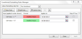
The next thing you’ll see by dissecting this template will show you how to use a check mark in a drop down list. Another function you can examine is how to use conditional formatting to color a cell based on the cell’s value. In this case, we want to color our cell green if it contains a check mark and red if left blank. As you can see, you will use the "ü" symbol in the formula.


There are similar online tools to help you schedule meetings but most require a fee to unlock all the features. Instead you can use and modify this free Excel template. You could add more functionality, like adding a formula to automatically send an email once you’ve picked the meeting time.

Do you think this template will be useful to you?

Wednesday, October 7, 2015

Excel Quick Tips: Count Unique Values

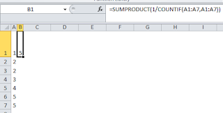
I’ve got an extremely short but valuable Excel tip for you today: how to count the number of unique values in a range. Sometimes you need to count values in a row or column but not if they repeat. To count only the unique numbers or words in Excel, use the following formulas depending on:

If there are no blank cells:

=SUMPRODUCT(1/COUNTIF(Range, Range))

With or without blank cells:

=SUMPRODUCT((Range<>"")/COUNTIF(Range,Range&""))

Replace Range with A1:A7 for example. 


COUNTIF is probably the function you’re most used to that will count based on a given condition. SUMPRODUCT returns the sum of the product in the range.  SUMPRODUCT functions as an array formula, you just don't have to enter it as such. 

To see how this formula works step by step, click on the cell that contains the formula, then go to Formula tab, and click Evaluate Formula and you can cycle through each step in the calculation.


For more, see the index of Excel tips page.