How do I insert the degree symbol in Microsoft Excel? (And other keyboard shortcuts)

There are a number of keyboard shortcuts that can be used to generate symbols in Excel spreadsheets. The most asked about one is how to insert the degree symbol. Here is a list of some of the most frequently used keyboard shortcuts:

Alt + 0176 = ° (Degrees)
Alt + 0149 = • (Bullet)
Alt + 0162 = ¢
Alt + 0188 = ¼
Alt + 0189 = ½
Alt + 0190 = ¾
Alt + 0177 = ±
Alt + 0178 = ²
Alt + 0179 = ³
Alt + 0163 = £
Alt + 0128 = €
Alt + 0151 = — (m dash)
Alt + 0150 = – (n dash)
Alt + 0187 = »
Alt + 0169 = ©
Alt + 0174 = ®
Alt + 0165 = ¥
Alt + 0177 = ±
Alt + 0247 = ÷
Alt + 0166 = ¦
Alt + 0134 = †
Alt + 0227 = ã
Alt + 0191 = ¿
Alt + 0161 = ¡
Alt + 0209 = Ñ
Alt + 0241 = ñ
Alt + 0225 = á
Alt + 0233 = é
Alt + 0237 = í
Alt + 0243 = ó
Alt + 0250 = ú
Alt + 0252 = ü
Alt + 0186 = ° (1° = primero)
Alt + 0170 = ² (2² = segunda)

As with most software these days, there are a number of different ways to get to the same result. You can also use character map to use the symbol you are looking for:

A character map of all special symbols, including foreign language characters, can be displayed by going to Start>Run, typing charmap, and clicking OK (Windows XP users). Vista users will type charmap into the Search window at the bottom of the Start Menu. Choose the font corresponding to the one you're using and click on a character. Next click Select>Copy to copy the character. Return to your document, click where you want the character inserted, and go to Edit>Paste (or do Ctrl+V) to insert it.

Finally, the simplest way is simply to where MSOffice users can go to Insert>Symbol to accomplish the exact same thing.

How do you automatically enable macros when Excel is opened?

•To automatically enable all macros when Excel is opened so you don’t have to do it manually every time, please read the following instructions:

1. In Excel, click the Office button in the upper left corner of the screen. 

 

  2. Click the "Excel Options" button in the lower right.

  

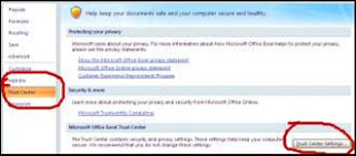
3. Click the "Trust Center" button on the left. Then, at the bottom right, select "Trust Center Settings" as shown below.

 

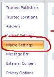
4. In the next window, select "Macro Settings," then select the radio button for “Enable all macros."

 

  There you have it! Now you don't have to enable the macros every single time that you open Excel.

How do I use a formula to count the remaining days until the end of the month in Excel?

Using the =DAY(TODAY()) commands I can get the date 2/15/2010 to show that we are on day 15 of the month. I would like the number all the way up to the last day of the month and then stay there. In this example November counted up to 30 days, Dec to 31, Jan to 31, and since today is the 15^th of Feb it is currently on 15. Tomorrow it will be 66. After the 31 I would like it to stop at 31. Is there a possible formula for this?

Month	Days
2009-Nov	30
2009-Dec	31
2010-Jan	25
2010-Feb	15

Yes there is a formula. First, you would need to have a fixed component or refer to a year/month value. Try this for January 2010:

=IF(--TEXT(TODAY(),"yyyymm")>201001,DAY(DATE(2010,2,0)),DAY(TODAY()))

That formula would begin by returning 1 on 01-JAN-2010 and increment by 1
each day up through 31-JAN-2010...then it would stay at 31

February 2010 would be this:

=IF(--TEXT(TODAY(),"yyyymm")>201002,DAY(DATE(2010,3,0)),DAY(TODAY()))

Now, one other thing you can do is take the 201002 numbers and place those in a separate column and then just point to that column in your formulas.

What do the hypens before TEXT do? A leading hyphen causes Microsoft Excel to interpret the contents of a cell as a formula. If you want to use a leading hyphen but not create a formula, use an en dash (option-hyphen) or an em dash (shift-option-hyphen) in place of the hyphen. Excel treats them like any letter or number.

You can also force Excel to treat the contents of any cell as text by typing an apostrophe at the beginning of the cell contents. Alternatively, format the cell as text (choose Cells from the Format menu, click the Number tab, and double-click Text in the category list). After changing a cell to text format, you may have to press command-U to make the change take effect.

Apostrophes (') and hyphens (-) are ignored, with one exception: If two text strings are the same except for a hyphen, the text with the hyphen is sorted last.

How do I create a week ending date formula for an expense report?

Let’s say you are putting together an expense report sheet for all of your employees to use. You want them to be able to enter a week ending date and the spreadsheet will automatically compute the rest of the dates for the week. Here are the two main formulas we will be using:

=IF(B1<>"",IF(WEEKDAY(B1)<>7,B1+7-WEEKDAY(B1),B1),"")

=IF($B$2<>"",$B$2-6,"")

First it says, if the date in cell B1 does not equal (< >) blank (“”), then go on to the next part of the formula, otherwise leave blank. The formula =weekday() returns a number 1 to 7 identifying the day of the week of date. In our example, I have chosen 2/12/2010 as the week ending date. =weekday(B1) turns out to be 6. So, if the weekday of B1, which is 6, does not equal 7, then take the value of B1, 12, add 7 to get 19, then subtract weekday of B1, 6. We end up at 13. (recap: 12+7=19. 19-6=13.) The date displayed is 2/13/2010.

Now it is on to the next formulas for each day. Sunday’s formula is: =IF($B$2<>"",$B$2-6,""). If B2 does not equal blank then subtract 6, otherwise leave blank. In our example we have 13-6=7 which gives us the correct date for Sunday, February 7, 2010. The formula for Monday is: =IF($B$2<>"",$B$2-5,"") which gives us 13-7=8 for Feb. 8th and so on until Saturday. There you have it, one easy way to improve your expense reports.

I could just put this up as templates and not even bother explaining how they work but how many people would take the time to try and figure out how they work? You will learn a lot and feel much more accomplished if you try building these spreadsheets on your own. Feel free to let me know if you have any questions or comments.

How do I highlight duplicate rows in Excel without deleting them?

There is a Delete Duplicates function in Excel that makes it very easy to delete any duplicate data in your spreadsheet. However, sometimes you may not want to delete that data, you just want to know that there are duplicates. One way of doing this is with a simple macro. To highlight and draw attention to duplicates in a Microsoft Excel spreadsheet with a bold red color create this macro (alt+F11 opens the macro editor):

Sub DupsinRed()
Application.ScreenUpdating = False
Rng = Selection.Rows.Count
For i = Rng To 1 Step -1
myCheck = ActiveCell
ActiveCell.Offset(1, 0).Select
For j = 1 To i
If ActiveCell = myCheck Then
Selection.Font.Bold = True
Selection.Font.ColorIndex = 3
End If
ActiveCell.Offset(1, 0).Select
Next j
ActiveCell.Offset(-i, 0).Select
Next i
Application.ScreenUpdating = True
End Sub

The statement "Application.ScreenUpdating = False" prevents the screen from updating to ensure the macro runs faster and the screen will not flicker. Don't forget to set it back to "True".

How do I create nested IFs formula or an IF in conjection with OR function?

IF/OR

To create a Microsoft Excel formula with an IF and an OR statement read the following example:

=IF(OR(E15=“ALUMINUM 2117”,E15=“STEEL ALLOY”), ”CADIUM PLATE”, ””)

If the text of cell E15 is exactly “ALUMINUM 2117” OR “STEEL ALLOY”, then the selected cell will display “CADIUM PLATE”, otherwise no value will be displayed because of the null set, or empty quotations at the end.

Nested IFs

You may need a formula that involves several IF statements in one. We call these IFs inside IFs Nested IFs (that's a lot of IF's!) See these examples:


=IF(C2=2,0.062, IF(C2=3, 0.094, IF(C2=4, 0.125, "")))

Explanation: If the value in cell C2 is equal to 2, then the dimension 0.062 will be displayed, if the cell C2 is equal to 3, 0.094 will be displayed, if cell C2 is 4, then 0.125 will be displayed, otherwise nothing will be displayed.
Make sure the number of left parentheses equals the number of right parentheses (color coded in Excel). Also note that Microsoft Excel 97-03 only allows users to have 7 levels of nested Ifs.

Other examples:

=IF(U17="CRES 303", "C", IF(U17="CRES A286", "CA", IF(U17="ALLOY STEEL", "-", "")))

=IF(C2=2,0.062, IF(C2=3, 0.094, IF(C2=4, 0.125, IF(C2=5, 0.156, IF(C2=6, 0.187, IF(C2=8, 0.25, ""))))))

Stay tuned for more!

Please feel free to ask any questions.