Podcast Analytics Tracking Spreadsheet

When the COVID-19 pandemic struck last year, many people were stuck at home with nothing to do so they started podcasting. As many of you may know, I love traveling to theme parks around the country. We had discussed starting a podcast for a site I also created content for, Coaster101.com, for years but it wasn’t until the midst of the global pandemic when we finally turned it into reality. Listen to me ramble about visiting amusement parks and riding roller coasters here: https://www.coaster101.com/podcast/

Once we got the hang of recording and it become a permanent thing, we started to analyze our analytics to try to decide what was working and what wasn’t. By understanding the data, you can make decision to help you grow your podcast. Like everything else I do, I decided to make a spreadsheet to track specific stats I had in mind. I’ve turned it into a template you can use, available to download for free here.

 As I always say, even if you don't have a direct use for this spreadsheet you can still learn something about Excel by examining this template.

For starters, it uses Ranking formulas in Excel to show the most popular and least popular episodes. As I do with almost all of my spreadsheets, I color code the columns so I can easily know which require manual data input by me, which are drop down lists, and which use formulas to be left alone. I use the TODAY() formula to help determine how many days old a podcast episode is (because one just released will obviously have fewer downloads than other episodes). You’ll see there are SUMIF and VLOOKUP formulas as well. Feel free to take a look:

Podcast Downloads Tracking Spreadsheet here

How to Add Conditional Formatting with a Macro

Conditional Formatting is a useful tool in Excel that allows you to do things like highlight duplicate cells, or color every other row in with color, and so on. If you have a large range or table with many conditional formatting rules, sometimes things can get a little messy. If you’re inserting, adding, or deleting rows and columns often, your conditional formatting rules might go from a short, highly understandable list, to a complete cluster:

One way to be able to reset your conditional formatting rules is with a macro. We’re going to use a macro to automatically delete the conditional formatting and then add it back.

First, to clear and delete all the conditional formatting from a sheet with a macro, use this code, changing the A:AQ with whatever range you’re using:

    '--------delete the conditional formatting--------

With ActiveSheet.Range("A:AQ")

    .FormatConditions.Delete

End With

Now it’s time to add conditional formatting with a macro. In this example, I have a status column C where I enter values, and based on these values the format of my range will change.

Use LastRow to find the last row of data, making it a dynamic range (meaning the size of the range changes based on how much data is inside the range).

'define the last row

LastRow = Cells(Rows.Count, 1).End(xlUp).Row

First, define the range where you want to apply the formatting.

Next, define the formula or rule. Here, I want if the value in Column C is the letter N to change the font color to red. I use double quotations to have a quotation. Notice there is only one $ sign. If I put $C$11 then the formula would not trickle down through the rest of the range.

Finally, define the condition, font color to red the color index is 3. See the font color index here: https://www.automateexcel.com/excel-formatting/color-reference-for-color-index/

This is the first rule I am adding so notice the (1) inside the parenthesis.

'-------add the conditional formatting-------

'if new, change font to red

  With ActiveSheet.Range("D11:AP" & LastRow)

     .FormatConditions.Add Type:=xlExpression, Formula1:="=$C11=""N"""

     .FormatConditions(1).Font.ColorIndex = 3

End With

 

Now I want to add another conditional formatting rule programmatically. This time, change the font color to green if there is an H in the column C. Green uses a 4 in the color index. This is the 2^nd rule so notice the (2).

 

'if h, change font to green

  With ActiveSheet.Range("D11:AP" & LastRow)

     .FormatConditions.Add Type:=xlExpression, Formula1:="=$C11=""h"""

     .FormatConditions(2).Font.ColorIndex = 4

End With

 

Finally, if there is an X in column C, I want to use strikethrough to cross out the words.

 

'if x, then cross-out

   With ActiveSheet.Range("D11:AP" & LastRow)

     .FormatConditions.Add Type:=xlExpression, Formula1:="=$C11=""x"""

     .FormatConditions(3).Font.Strikethrough = True

End With

 Here's what the conditional formatting rules look like after running the macro:

And that’s how you add conditional formatting with a macro. Let me know in the comments below if you have any questions.

How to Make a Drop Down List From a Macro

Drop down lists in Excel are super helpful when you want to limit a user’s input to a set of predetermined choices. Normally, drop down lists can be made by clicking on a cell, going to the data tab, then by using the Data Validation function. Change Allow to List. 

But what if you’re importing data from another Excel file and want to automatically create a drop down list? It’s possible to do using VBA. To create a drop down list from a macro in cell A1, try this code in the VBA editor:

 

Sub ListCreator()

Range("A1").Validation.Add Type:=xlValidateList, AlertStyle:=xlValidAlertStop, _ Formula1:="OK,Maybe,No"

End Sub

 

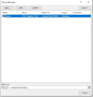
Here, all the entries in the list will be created from the macro. What if one of the entries needs to change? Only someone with VBA experience will probably be able to figure out how to change it. So I like to create the list somewhere within the spreadsheet where anyone can see it and it’s obvious what it’s used for, then use the Name Manager to create a Named Range to easily refer to the list. This way, if you decide to add entries later the lists will automatically be updated as long as they used the Named Range.

 

In this example, I select my list within the Excel sheet (column G), and give it the name “Status”.

To used a Named Range when you create a drop down list via VBA, simply refer to the Named Range:

 

Range("A2").Validation.Add Type:=xlValidateList, AlertStyle:=xlValidAlertStop, Formula1:="=Status"

 

To set a default value, simply set the value of the cell after changing the data validation:

 

Range("A2").Validation.Add Type:=xlValidateList, AlertStyle:=xlValidAlertStop, Formula1:="=Status"

 

Range("A2").Value = “OK”

 

It might be easier to understand by watching this short video:

 

That’s all there is to it! Now you know how to add a drop down list from a macro in Excel. How often do you use drop down lists? I’d love to know, so let me know in the comments below.