Typically, to transfer horizontal rows into vertical columns in Excel you would highlight the cells you want to change and copy, then right click on the cell you want to move to, select ‘paste special’, click ‘transpose’ box, and hit ok. But what if you want to accomplish this task with a formula instead so it is done automatically on the fly? In an earlier post I showed you how to do it by using the OFFSET function combined with a named range. Today, I’m going to show you a different Excel formula to transfer rows to columns.
It takes all the names in row 39 on the Master Pool sheet from column J to Z and puts them into a vertical column in the leaderboard sheet, starting in row 3. The dollar signs are very important. As you fill the formula down the range increases. I also used the IF and ROW functions to account for the number of players (if the row number minus two, because the formula started in row 3, is less than or equal to the total number of players, then transpose the data, otherwise leave blank). As you can see in the example spreadsheet, the data is transformed from a horizontal row on one sheet to a vertical column in another. This is important because the data in the horizontal column can change and the vertical column will update automatically - no manual revisions needed!
I recently used these horizontal to vertical formulas in my 2013 NCAA college football bowl prediction pool manager, and I am going to refer to that template as an example, so if you haven’t already I recommend you download the sheet. I needed to get the list of the players from the main sheet, which were listed out horizontally, and get them into the leaderboard sheet. The players needed to be listed vertically in the leaderboard in order for my rank without ties formula to rank the players in order of who picked the most games correctly. The basic formula uses INDEX and ROWS functions and looks something like this:
=INDEX(Sheet2!D$22:H$22,ROWS(A$4:A4))
The INDEX function returns the value of the cell at the intersection of the rows and columns specified in the formula while ROWS returns the number of rows in a reference or array. The exact formula I used on the leaderboard sheet in cell A3 is shown below:
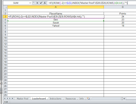
=IF((ROW()-2)<=$L$3,INDEX('Master Pool'!J$39:Z$39,ROWS(A$4:A4)),"")
 |
| The formula - notice the range |
 |
| The range expands as the formula is filled down |
It takes all the names in row 39 on the Master Pool sheet from column J to Z and puts them into a vertical column in the leaderboard sheet, starting in row 3. The dollar signs are very important. As you fill the formula down the range increases. I also used the IF and ROW functions to account for the number of players (if the row number minus two, because the formula started in row 3, is less than or equal to the total number of players, then transpose the data, otherwise leave blank). As you can see in the example spreadsheet, the data is transformed from a horizontal row on one sheet to a vertical column in another. This is important because the data in the horizontal column can change and the vertical column will update automatically - no manual revisions needed!
This horizontal-to-vertical formula guide is super useful! Automatically transposing data with INDEX and ROWS makes managing large spreadsheets much easier. For anyone who also plays mobile games and wants to track stats efficiently, the raid shadow legends helper is a great tool to streamline progress tracking.
ReplyDelete